

The Weak and Strong Form of "AI for Science"
From physics-informed to physics-enforced


AI for Science’s Pursuit of Dimension-independence
Many challenges in scientific computing and applied mathematics involve dealing with high-dimensional problems. This high dimensionality often arises from multiscale effects. For example, the dimensionality of quantum many-body systems grows exponentially with the number of electrons included. And microscopic scale models in multiscale modeling often have a very large number of degrees of freedom. The difficulties caused by excessive dimensions are also known as the “curse of dimensionality”.
Traditional smoothness regularization methods clearly fail in high dimensions, unable to effectively describe the complexity of functions. Recent research has shown that approximating functions with specific neural network architectures provides a better measure of complexity. This has led to new function spaces associated with particular machine learning models, such as RKHS and Barron spaces, laying new foundations for analyzing high-dimensional function approximation. Meanwhile, machine learning models themselves have demonstrated powerful capabilities in approximating high-dimensional functions, enabling solutions to many previously intractable control theory and PDE problems due to the curse of dimensionality.
Various AI algorithms, including reinforcement learning and transfer learning, are not only expanding the scope of AI4Science models through continuous optimization and improvement, but also reducing model training costs. In the computer age, we often solve real-world problems by mapping physical models onto computers for mathematical simulation. However, more microscopic models, although more accurate as they are closer to first principles, face more severe “curse of dimensionality” due to their greater complexity and larger number of degrees of freedom. In contrast, more macroscopic models are simpler, more efficient, but less accurate. In this case, we need to find a way to reduce computational complexity while maintaining accuracy.
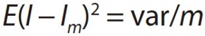
In statistical physics, the Monte Carlo method is a solution to this “curse of dimensionality” (see equation below). Its convergence efficiency in sampling depends on the variance of the function and the number of samples, but not the input dimension, thus making it dimension-independent.
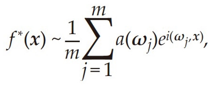
In the AI4Science era, neural network functions (see equation below) have properties similar to Monte Carlo methods. For function spaces we care about, approximation errors depend on intrinsic variances related to the function rather than the dimensionality of the function.
Leveraging this trait of AI algorithms, we can use them as bridges between multiscale physical models, effectively approximating solutions of microscopic models. This allows microscopic models to become data generators, then through learning under AI, fuse corresponding models into more macroscopic ones. Through such iterative interactions, we can find a solution balancing microscopic accuracy and macroscopic efficiency. Using neural networks to approximate the policy function in dynamic programming can solve stochastic control problems with hundreds or even higher dimensions. Solving high-dimensional Hamilton-Jacobi-Bellman equations also becomes promising[1].
In practice, how to build bridges between AI and science is the core innovation point. Currently, the approaches differ for various scientific scenarios. In control problems, the goal is to find a policy function that optimizes an objective function (usually integral of state trajectories). Traditional dynamic programming methods need to solve a Bellman equation with dimension equaling the state space dimension, thus facing the curse of dimensionality. To address this, researchers propose representing the policy function with neural networks, viewing the control objective as a loss function, and the control dynamics as constructing a deep residual network. The network parameters can then be trained using stochastic gradient descent. Such deep learning control algorithms can already handle stochastic control problems with over a hundred or even higher dimensions. The Hamilton-Jacobi-Bellman (HJB) equation also plays a core role in control theory. In recent years, progress has been made in solving high-dimensional HJB equations using adaptive deep learning algorithms. This enables better handling of complex control problems in continuous state spaces.
In multiscale modeling, microscopic models contain too many details to be directly used for practical simulations. And traditional uniform spatial discretization algorithms also struggle to handle such high-dimensional microscopic models. Machine learning methods can identify macroscopic or collective variables from microscopic simulations, establishing connections between different scales and enabling direct multiscale coupling. Recent research shows this approach can extend atomic-level simulations to systems containing over a billion atoms.
For building physical models from data, machine learning also provides new ideas. Merely fitting data is not enough. Physical constraints need to be combined and training should use representative data, so that the model is interpretable and guarantees extrapolability. This brings hope to many problems that are hard to model starting from general physical principles. As long as physical constraints are satisfied, such models can achieve reliability comparable to general physical models.
3 Levels of “Enforcing” Physical Constraints onto Machine Learning’s “Black box”?
Classical AI: From the perspective of "classical AI", improving a model's physical fidelity mainly comes from enhancing the quality of its training data. This is the weakest form, simply embedding physical knowledge into the training data itself. For example, generating data satisfying conservation laws or known symmetries for training. Such end-to-end utilization of data for modeling is fast and easy, but cannot guarantee the model will obey physical laws during inference.
“Physics-informed”: A soft form is indirectly strengthening physical laws through the loss function. For example, Physics-informed Neural Network (PINN) incorporates differential equations into part of the loss function, guiding parameter optimization. PINNs embed differential equations and other physical constraints into the neural network structure to approximate functions containing physical laws. The inputs to a PINN include independent variables x and parameters λ, and the output is the solution u(x,λ). Network parameters are trained by minimizing a loss function consisting of two parts: 1) Data fitting - using network output u(x,λ) to approximate given data; 2) Physical constraints - taking derivatives of u(x,λ) and substituting into differential equations to require satisfying the equations. This is implemented via automatic differentiation. After training, the lowered loss function means an u(x,λ) satisfying both data and physical constraints is found. Variational methods also belong here, optimizing a functional (such as action in classical mechanics or free energy in statistical mechanics). Such forms can partially constrain the model, but will not rigidly require obeying physical principles.
“Physics-enforced”: A stronger form directly builds fundamental physical laws into the model architecture. Using descriptors preserving problem symmetries is a typical example. Another is constructing Hamiltonian or Lagrangian neural networks with structures respecting certain physical conservation laws like energy. This form maximally ensures model behaviors conform to physical principles, but also restricts model expression. In DeePMD, researchers cleverly incorporated some key physical constraints: 1) Translation invariance - the total energy of a physical system does not depend on absolute atomic positions. This is achieved by expressing the system energy as a sum over atomic energies, each determined by the atom's local environment defined relative to the atom, thus ensuring translational invariance. 2) Rotation invariance - the total energy should not change under system rotations. DeePMD implements this by using rotationally invariant local descriptors. 3) Permutation invariance - swapping atom indices should not change the total energy. DeePMD also guarantees this through summing atomic energies. These invariances are key components of the DeePMD design. The model is trained on potential energy surfaces from quantum mechanics calculations. The invariances help ensure the learned model can generalize well to new systems. Without them, the model would struggle to predict properties of systems different from the training data.
It should be emphasized that stronger physical constraints are NOT “better” by default, but depend on the specific factors for each case (such as data quality, and the end user’s actual expectation). For example, AlphaFold does not impliment very strong constrains, yet thanks to the extremely high quality of the PDB data source, its training is very successful, with excellent inference performance and efficiency. Meanwhile, introducing strong L2 constraints sometimes decreases model trainability, impacting time and cost. When constructing AI for Science algorithms for specific scenarios, pragmatism is always a good idea.
Advances in AI for Science depend not only on applying AI algorithms, but also on improving and enhancing many classical algorithms. With the lowering of barriers to acquiring high-quality and large-scale data, how to better fuse data from different sources, scales, and modalities has become an important challenge. For example, in weather forecasting, the spatiotemporal scales corresponding to different observed indicators have large differences. How to utilize such data with differences to enable more accurate and efficient forecasting poses real algorithmic challenges, requiring us to improve classical data fusion algorithms to adapt to new demands. The tremendous imagination space for AI for Science lies in how to better utilize AI algorithms to connect scientific computing and physical models, guiding scientific and industrial innovation. The power of AI lies in its great potential to solve complex problems, thus advancing scientific research and technological development.
Today, the bottleneck in research is not only "how to solve problems", but also "how to define problems" and "how to choose tools". For example, when solving PDEs, if the main difficulty is high dimensionality, PINN would be very effective. But if the challenges do not lie in the curse of dimensionality, but rather geometrical complexity, multiscale effects, etc., the advantages of neural networks would not easily emerge. Instead, difficulties like nonlinear optimization would lead to low solving efficiency, uncontrollable errors, and difficulty improving systematically. In such scenarios, choosing the Random Feature Method (RFM) could avoid mesh generation and easily handle complex geometries.

Deep understanding of the problem is the first step to solving it. The innovations in AI for Science algorithms come not only from the ever-changing AI models, but even more so from scientists' analysis, diagnosis and “translation” of specific scientific challenges, in order to maximize the effectiveness of AI in the scientific domain.
Source:
[1] Weinan E, "The dawning of a new era in applied mathematics" , Notice of the American Mathematical Society, April, 2021.
[2] Jingrun Chen, Xurong Chi, Weinan E & Zhouwang Yang. (2022). Bridging Traditional and Machine Learning-Based Algorithms for Solving PDEs: The Random Feature Method. Journal of Machine Learning. 1 (3). 268-298. doi:10.4208/jml.220726